A Primer on Electrical Mismatch
 Figure 1: Google’s Gemini’s creative-ish take on what shading electrical mismatch looks like.
Introduction
Electrical mismatch due to non-uniform shading can be a confusing topic for both new and experienced PV performance modeling professionals. This is understandable due to the fact that learning about mismatch requires building up layers of intuition from multiple fields including PV performance modeling, PV systems design, materials science, and electrical engineering. In this joint(!) blog post, Mark Mikofski and I will guide you around some common misconceptions that arise when talking about electrical mismatch due to non-uniform shading.
Misconception 1: PV performance modelers enter a percentage value in their modeling software to model the effects of mismatch due to shading
The reality is that there are many different causes of mismatch that can occur in an operating solar power plant. For example, electrical mismatch due to non-uniform shading, non-uniform dust & snow soiling, non-uniform wire distances, etc. This misconception arises because array level mismatch is often modeled as a percentage in module quality, but electrical mismatch due to shade is never modeled in module quality.
Array level mismatch
The first type occurs when modules with difference efficiencies are included in the same array. For example, a company may buy a set of 500W modules and install them in a strings of 28 modules each. If each of these modules actually performed at 500W at STC, there would be no mismatch, but in reality each will perform slightly differently due to differences in materials and manufacturing. In order to reduce this effect, manufacturers bin their modules so that they come in a set where all modules in the set fall within a given tolerance. Using our 500W module example from before, the company may receive 10,000 modules all within a 500W to 505W bin. Large PV projects may receive modules across multiple bins and must be careful to string modules with similar power bins together. So even if current mismatch is reduced by binning within strings, there may still be voltage between strings due to these manufacturing differences in module efficiency. In a PV performance model, the actual power ratings are generally considered to be normally distributed, and the loss associated is generally a flat percentage across all time-steps. This type of mismatch is often called array or system-level mismatch, is always a loss, was documented by Louis L. Bucciarelli Jr. in 1979, and has been reported by various researchers between 0.5% to 2% for typical PV systems. PV performance modelers can calculate this value from flash test data and use it as in input into their PV performance modeling software. However, in this blog post we will ignore array level mismatch in favor of electrical mismatch due to shading.
Electrical mismatch due to shade
The other type of mismatch loss that is calculated in a given performance modeling software occurs due to shading. This type of shading is generally modeled in conjuction with the performance modeling software’s shading model, and is not modeled as a flat loss. (Read more in my post about modeling shade.)
Shade modeling is complex because the electrical behavior of the PV string changes depending on the direction of the shade. In this blog post we will explore row-to-row shade which partially covers all modules by the same amount, and in Mark’s joint post he will use modeling to examine what happens when non-uniform shade from a tree, a turbine mast, or a transmission tower crosses over only a subset of cells or modules.
The physical causes and intuition for all sources of mismatch are the same and learning about one source of mismatch is instructive in modeling the other sources as well. However, a guide to help you to understand and remember these three types of mismatch is to reduce them to the variables that affect each most:
Array level mismatch is caused by random differences throughout the system.
Row to row mismatch is governed by the fraction of modules shaded, which is constant for all modules in the string. It generally looks like the image below.
 Figure 2: InterRow Shading.
Non-uniform shade is characterised by the number of parallel strings the shadow crosses (generally orthogonal to row to row shade).
Building up the Intuition
Talking about mismatch can be difficult since every engineer has a different level of understanding of each of the multitude of fields that underpin the effect. Very few undergraduate programs feature coursework in PV performance modeling, and new-comers to the field usually come familiar with one of the following fields, but not all of them (electrical engineering, mechanical engineering, chemical engineering, materials science, structural engineering, physics, etc.). The following few sections of the post are useful to level set for the many different types of engineers that may be reading this post, though please feel free to skip any sections that you are already very familiar with.
PV Systems Design
Some terminology:
- Cell: For the purposes of this blog post, silicon doped to create a PN junction and separated from other cells by wires.
- Module: A collection of electrically connected cells (generally 72 for utility scale plants)
- Sub-Module: A set of cells which are connected in series, and connected to a bypass diode in parallel. Sub-modules are connected to each other in series.
In large utility scale solar power plants, many strings of module are generally connected to an inverter with a single maximum power point tracker (MPPT) or very few MPPTs relative to the number of strings.
Misconception 2: As soon as a module is shaded, production goes to zero
I have heard this misconception quite a bit, especially when working in the residential sector. In a photovoltaic performance models, there are 3 different types of irradiance that hit the front side of a solar module: beam, diffuse and ground reflected. For now we will ignore the circumsolar portion (which generally gets bucketed into either the beam or diffuse portions), as well as the ground reflected irradiance which is generally considered to have an isotropic-ish effect much like the diffuse portion.
Beam irradiance is the most intuitive of the irradiance types and can be thought of as light which takes a direct (straight vector) path from the sun to the solar module. Beam irradiance can be blocked by any object that sits between an object and the straight vector pointing to the sun position. Blocking objects may include trees, buildings, or other solar modules.
Diffuse irradiance on the other hand is less intuitive and encapsulates all of the light that hits a module, but does not take a direct line from the sun. For example, a photon may bounce off of the ground, then a molecule in the atmosphere, and then be directed towards the module (horizon brightening). The cumulative effect of many photons all taking circuitous paths to the module results in a “diffuse dome” of irradiance which can be integrated to determine how much diffuse light is hitting the module. It is this diffuse irradiance which makes it so that if so that objects in shade are still visible. An illustration below from PVEducation.
 Figure 3: Diffuse Dome.
The module power cannot go to zero since some diffuse light still shines on the module. In Desert Center, CA (a location with a very low fraction of diffuse light energy relative to direct light energy) the proportion of total irradiance due to diffuse light in the plane of the array on a tracker system is around 18%.
Electrical Engineering
This blog post assumes that the reader has taken entry level electrical engineering and materials science curriculum at the university level, but that a refresher may be useful. Those with a need for a refresher on the material science of solar cells, including forward and reverse bias will find this video series informative [4].
Some rules to remember:
- Voltage adds in series.
- Current adds in parallel.
- Current into and out of a node must sum to zero.
- Voltage in a loop must sum to zero
- Diodes allow current to pass in one direction during normal operation.
- Diodes allow current to pass in the opposite direction at a threshold negative voltage.
- Both PV cells and bypass diodes are modeled as diodes.
- A current source can be thought of as a device which supplies a constant current at a range of different voltages.
- A voltage source can be thought of as a device which supplies a constant voltage at a range of different currents.
 Figure 4: A general diode IV curve from LibreTexts [1]
What is an IV curve? It is a continuous curve which represents all of the possible output states that the solar string can operate at. The lower limit at Isc represents the output in the string if the circuit is completed with an “element” of zero resistance. The upper limit of Voc occurs if the string is completed with an infinite resistance. Interested readers can refer to more information in [5]. A maximum power point tracker (MPPT) modulates the resistance between these two limits to find the maximum power point. Why do we care about the IV curve?
Quoting Mark Mikofski [2]:
The cells in a PV module can be considered roughly as a current source in parallel with a diode and some resistive elements. Diodes are semiconductors. In other words, they only conduct current in one direction, called the forward bias. When a negative voltage, or a reverse bias, is applied to the cell, the semiconductor won’t conduct a current. However, if enough reverse bias is applied, all semiconductors will eventually breakdown, and carry a current. This phenomema is called reverse bias breakdown, and the breakdown voltage varies between cell technology. A typical front contact p-type silicon solar cell may breakdown at around -20 volts, while a back-contact n-type silicon solar cell may breakdown at -5 volts. There are many factors, beyond the scope of this primer, that affect reverse bias breakdown, such as purity of the substrate as well as type and concentration of dopant. The most important thing to understand about reverse bias breakdown is this: When a cell is in reverse breakdown, it can carry nearly any current, but because the voltage is negative, then the cell will dissipate energy and will get hot as it exchanges heat with the environment around it.
So why would a negative voltage be applied to a cell? A cell that is shaded on its own does not enter reverse bias. Neither does a cell which is in a string with similarly shaded cells. Therefore in order for reverse bias to occur there must be a mismatch in the current and voltage characteristics in one of the cells of the string relative to the others. Why does this mismatch cause a reverse bias? Well, lets closely examine what we said earlier when we stated that the cells in a module can be “roughly” considered as a current source.
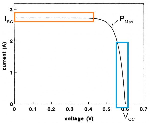 Figure 5: IV Curve.
In the orange region above it is true, the solar cell is behaving like a current source, and is providing a steady current at a range of different possible voltages. In the blue region the cell behaves more like a voltage source which holds a steady-ish voltage, but supplies a range of possible currents. Here is an image comparing the output of a solar cell at different level of irradiance.
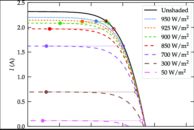 Figure 6: IV Curve at Different Irradiance Levels.
A shaded solar cell cannot, on its own, provide the same level of current and voltage as its unshaded counter-parts. As an example, lets say that in a series string of 10 1V cells that 9 are unshaded and 1 is shaded. These cells are connected into a circuit over a resistive load with a non-zero, non-infinite resistance. The 9 unshaded cells are experiencing forward bias due to the light hitting them, creating a potential of 9V. Kirchoff’s voltage law (voltage in a loop must sum to zero) then forces a ~ -9V potential across the shaded cell and the resistive load. This is the source of the reverse-bias.
Quoting PVEducation [3]:
If the operating current of the overall series string approaches the short-circuit current of the “bad” cell, the overall current becomes limited by the bad cell. The extra current produced by the good cells then forward biases the good solar cells. If the series string is short circuited, then the forward bias across all of these cells reverse biases the shaded cell. Hot-spot heating occurs when a large number of series connected cells cause a large reverse bias across the shaded cell, leading to large dissipation of power in the poor cell. Essentially the entire generating capacity of all the good cells is dissipated in the poor cell. The enormous power dissipation occurring in a small area results in local overheating, or “hot-spots”, which in turn leads to destructive effects, such as cell or glass cracking, melting of solder or degradation of the solar cell. Also
Bypass diodes allow this current that would otherwise flow throught the shaded solar cell to flow in an external circuit instead. Quoting PVEducation again [5]:
A bypass diode is connected in parallel, but with opposite polarity… Under normal operation, each solar cell will be forward biased and therefore the bypass diode will be reverse biased and will effectively be an open circuit. However, if a solar cell is reverse biased due to a mismatch in short-circuit current between several series connected cells, then the bypass diode conducts, thereby allowing the current from the good solar cells to flow in the external circuit rather than forward biasing each good cell.
Putting it all together
Electrical Mismatch
Starting from the very beginning: What does an unshaded system’s IV curve look like?
 Figure 7: Unshaded curve of 20 string system made my Mark Mikofski using PVMismatch.
What happens if we shade a single solar cell? Since current is proportional to irradiance, current is decreased.
Now what happens if we connect this shaded cell to another unshaded cell in series? Then the string is limited by the Isc of the shaded solar cell and excess power is dissipated in the shaded cell.
Then if we connect these cells into a module and then this module into a string? And all strings are shaded in the exact same way? Then every string gets limited to its most shaded cell and can only export the amount of energy incident upon the module by the diffuse irradiance.
But what happens if all strings are not shaded in the exact same way? What happens if the shade occurs perpendicular to the portrait mode modules instead of parallel to their long axis? Believe it or not, here is the IV curve of the shaded system.
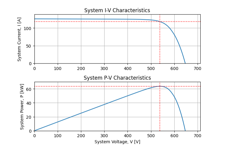 Figure 8: Shaded curve of 20 string system made my Mark Mikofski using PVMismatch.
Misconception 3: Only current is affected in partial shading situations”
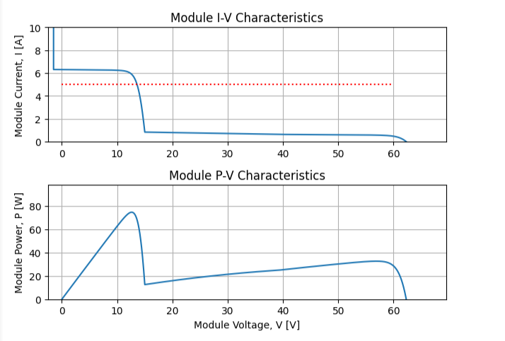
In Mark’s blog post which I highly suggest you hop over and read, he shows that, yes the module IV curve gets distorted by the shading. In the picture below, you can see that bypass diodes have indeed been activated, and the module can only export the 5A required by the string at ~13ish volts.
Why does the system curve look so different from the module curve? Each of the unshaded modules in the 20 string system operates at a slightly higher voltage than their individual maximum power point to make up for the lost voltage of the shaded module.
Conclusion
In real life, shade happens in many directions: along the module axis, perpendicular to the module axis, diagonal to the module axis… you get the picture. Two blog posts certainly won’t cover everything you need to know about electrical mismatch due to shading, but I hope that this information is helpful to give performance modelers some more intuition about how shade affects their systems.
From Mark: “I wish I could say, that’s all there is to it, but as I said in my first blog post, electrical mismatch in crystalline silicon is very counter-intuitive. That’s why I created PVMismatch to begin with. I was tired of guessing and being wrong. So don’t guess. Simulate with confidence, try PVMismatch, and let me know what you learn!”
Further reading: